Posts on psychometrics: The Science of Assessment

discrimination-parameter

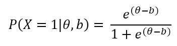
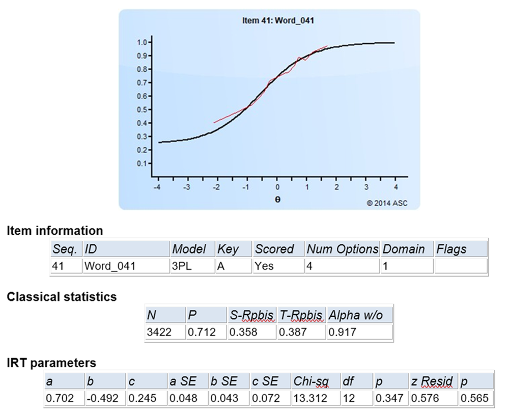
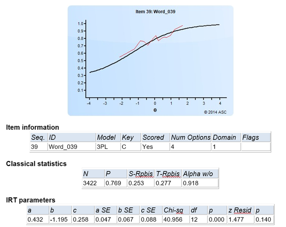
The item discrimination parameter a is an index of item performance within the paradigm of item response theory (IRT).  There are three item parameters estimated with IRT: the discrimination a, the difficulty b, and the pseudo-guessing parameter c. The item parameter that is utilized in two IRT models, 2PL and 3PL, is the IRT item discrimination parameter a.

Definition of IRT item discrimination

irf_b_-2.2

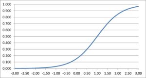
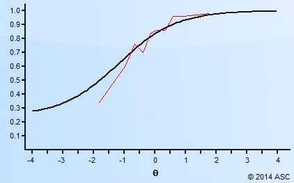
Generally speaking, the item discrimination parameter is a measure of the differential capability of an item. In the analytical aspect, the item discrimination parameter a is a slope of the item response function graph, where the steeper the slope, the stronger the relationship between the ability θ and a correct response, giving a designation of how well a correct response discriminates on the ability of individual examinees along the continuum of the ability scale. A high item discrimination parameter value suggests that the item has a high ability to differentiate examinees. In practice, a high discrimination parameter value means that the probability of a correct response increases more rapidly as the ability θ (latent trait) increases.

­­In a broad sense, item discrimination parameter a refers to the degree to which a score varies with the examinee ability level θ, as well as the effectiveness of this score to differentiate between examinees with a high ability level and examinees with a low ability level. This property is directly related to the quality of the score as a measure of the latent trait/ability, so it is of central practical importance, particularly for the purpose of item selection.

Application of IRT item discrimination

Theoretically, the scale for the IRT item discrimination ranges from –∞ to +∞ and its value does not exceed 2.0. Thus, the item discrimination parameter ranges between 0.0 and 2.0 in practical use.  Some software forces the values to be positive, and will drop items that do not fit this. The item discrimination parameter varies between items; henceforth, item response functions of different items can intersect and have different slopes. The steeper the slope, the higher the item discrimination parameter is, so this item will be able to detect subtle differences in the ability of the examinees.

The ultimate purpose of designing a reliable and valid measure is to be able to map examinees along the continuum of the latent trait. One way to do so is to include into a test the items with the high discrimination capability that add to the precision of the measurement tool and lessen the burden of answering long questionnaires.

However, test developers should be cautious if an item has a negative discrimination because the probability of endorsing a correct response should not decrease as the examinee’s ability increases. Hence, a careful revision of such items should be carried out. In this case, subject matter experts with support from psychometricians would discuss these flagged items and decide what to do next so that they would not worsen the quality of the test.

Sophisticated software provide more accurate evaluation of the item discrimination power because they take into account responses of all examinees rather than just high and low scoring groups which is the case with the item discrimination indices used in classical test theory (CTT). For instance, you could use our software FastTest that has been designed to drive the best testing practices and advanced psychometrics like IRT and computerized adaptive testing (CAT).

Detecting items with higher or lower discrimination

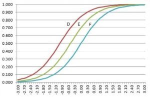
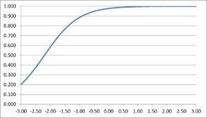
Now let’s do some practice. Look at the five IRF below and check whether you are able to compare the items in terms of their discrimination capability.

item response function

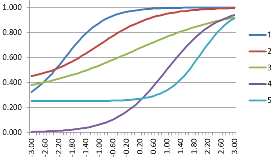
Q1: Which item has the highest discrimination?

A1: Red, with the steepest slope.

Q2: Which item has the lowest discrimination?

A2: Green, with the shallowest slope.


item-difficulty-parameter

The item difficulty parameter from item response theory (IRT) is both a shape parameter of the item response function (IRF) but also an important way to evaluate the performance of an item in a test.

Item Parameters and Models in IRT

There are three item parameters estimated under dichotomous IRT: the item difficulty (b), the item discrimination (a), and the pseudo-guessing parameter (c).  IRT is actually a family of models, the most common of which are the dichotomous 1-parameter, 2-parameter, and 3-parameter logistic models (1PL, 2PL, and 3PL). The key parameter that is utilized in all three IRT models is the item difficulty parameter, b.  The 3PL uses all three, the 2PL uses a and b, and the 1PL/Rasch uses only b.

Interpreting the IRT item difficulty parameter

The b parameter is an index of how difficult the item is, or the construct level at which we would expect examinees to have a probability of 0.50 (assuming no guessing) of getting the keyed item response. It is worth reminding, that in IRT we model the probability of a correct response on a given item Pr (X) as a function of examinee ability (θ) and certain properties of the item itself. This function is called item response function (IRF) or item characteristic curve (ICC), and it is the basic feature of IRT since all the other constructs depend on this curve.

The IRF plots the probability that an examinee will respond correctly to an item as a function of a latent trait θ. The probability of a correct response is a result of the interaction between the examinees’ ability θ and the item difficulty parameter b. With the IRF, as the θ increases, there is a rise in probability that the examinee will provide a correct response to an item. The b parameter is a location index that indicates the position of the item functions on the ability scale, showing how difficult or easy a specific item is. The higher the b parameter is, the higher the ability required from an examinee to have a 50% chance of getting an item correctly. Difficult items are located to the right or to the higher end of the ability scale while easier items are located to the left or to the lower end of the ability scale. The typical values of the item difficulty range from −3 to +3, items whose b values are near −3 will correspond to items that are very easy, whilst items with values near +3 will correspond to the items that are very difficult for the examinees.

You can interpret the b parameters as a sort of “z-score for the item.”  If the value is -1.0, that means it is appropriate for examinees at a score of -1.0 (15th percentile).

The b parameter interpretation for difficulty is the opposite of the item difficulty statistic p-value in classical test theory (CTT), where a low b indicates an easy item, and a high b indicates a difficult item. Obviously, higher b require higher θ for a correct response.  With the CTT p-value, a low value is hard and a high value is easy.  For this reason it is sometimes called item facility.

Examples of the IRT item difficulty parameter

Let’s consider an example. There are three IRFs below for three different items D, E, and F. All three items have the same level of discrimination but different item difficulty values on the ability scale. In the 1PL, it is assumed that the only characteristic that influences examinee performance is the item difficulty (b parameter) and all items are equally discriminating. The b-values for the items D, E, and F are −0.5, 0.0, and 1.0 respectively. Item D is quite an easy item. Item E represents an item of medium difficulty such that the probability of a correct response is low at the lowest ability levels and near 1 at the highest ability levels. Item F introduces a hard item with the probability of correctly responding examinees being low along the most of the ability scale and only increasing at the higher ability levels.

three item response functions D E F

Look at the five IRFs below and check whether you are able to compare the items in terms of their difficulty. Below are some specific questions and answers for comparing the items.

item response function

  • Which item is the hardest, requiring the highest ability level, on average, to get it correct?

Blue (No 5), as it is the furthest to the right.

  • Which item is the easiest?

Dark blue (No 1), as it is the furthest to the left.

How do I calculate the IRT item difficulty?

You’ll need special software like Xcalibre.  Download a copy for free here.

one-parameter-logistic-model

The One Parameter Logistic Model (OPLM or 1PL or IRT 1PL) is one of the three main dichotomous models in the Item Response Theory (IRT) framework. The OPLM combines mathematical properties of the Rasch model with the flexibility of the Two Parameter Logistic Model (2PL or IRT 2PL). In the OPLM, difficulty parameters, b, are estimated and discrimination indices, a, are imputed as known constants.

Background behind the One Parameter Logistic Model

IRT employs mathematical models assuming that the probability that an examinee would answer the question correctly depends on their ability and item characteristics. Examinee’s ability is considered the major individual characteristic and is denoted as θ (“theta”); it is also called the ability parameter. The ability parameter is conceived as an underlying, unobservable latent construct or trait that helps an individual to answer a question correctly.

These mathematical models include item characteristics also known as the item parameters: discrimination (a), difficulty (b), and pseudo-guessing (c). According to IRT paradigm, all item parameters are considered to be invariant or “person-free”, i.e. they do not depend on examinees’ abilities. In addition, ability estimates are also invariant or “item-free” since they do not depend on the set of items. This mutual independence forms the basis of the IRT models that provides objectivity in measurement.

The OPLM is built off only one parameter, difficulty. Item difficulty simply means how hard an item is (how high does the latent trait ability level need to be in order to have a 50% chance of getting the item right?). b is estimated for each item of the test. The item response function for the 1PL model looks like this:

One-parameter-logistic-model-IRT

where P is the probability that a randomly selected examinee with ability θ will answer correctly a specific item; e is a mathematical constant approximately equal to 2.71828, which is also known as an exponential number or Euler’s number.

Assumptions of the OPLM

The OPLM is based on two basic assumptions: unidimensionality and local independence.

  • Unidimensionality assumption is the most common, but the most complex and restrictive assumption for all IRT models that sometimes cannot be met. It states that only one ability is measured by the set of items in a single test. Thus, it assumes that a single dominant factor should underlie all item responses. For example, in a Math test examinees need to possess strong mathematical abilities to answer test questions correctly. However, if test items measure another ability, like verbal, this test is no longer unidimensional. The unidimensionality can be assessed by various methods, but the most popular among all is the factor analysis approach which is available in the free software MicroFACT.
  • Local independence assumes that in case of a constant ability, examinee’s responses to any items are statistically independent, i.e. the probability that an examinee would reply correctly to a test question does not depend on their answers to other questions. In other words, the only factor influencing examinee’s responses is the ability.

Item characteristic curve

The S-shaped curve describing the relationship between the probability of an examinee’s correct response to a test question and their ability θ  is called item characteristic curve (ICC) or item response function (IRF). In a test, each item will have its own ICC/IRF.

Typical ICC for the One Parameter Logistic Model looks like this:

irf_b_1.0

The S-shaped curve shows that the probability of a correct response is near zero at the lowest level of examinee’s ability and increases up to the highest level of ability as the probability of correct response approaches 1. The curve rises rapidly as we move from left to right and is strictly monotonic.

The OPLM function ranges between 0 and 1. ICC can never reach and cannot be higher than 1. Theoretically, item parameter ranges from -∞ to + ∞ but practically this range is limited between -3 and +3. You can easily plot ICC using the IRT calibration software Xcalibre.

Application of the OPLM in test development

The OPLM is especially useful in item selection, item banking, item analysis, test equating, and investigating item bias or Differential Item Functioning (DIF). Since the IRT One Parameter Logistic Model allows estimating item parameters that are “examinee-free”, then it is possible to estimate item parameters during their piloting to use them later. Based on the information about items and examinees collected during tests it is easy to build item banks that can be ultimately used for large-scale testing programs and Computerized Adaptive Testing (CAT).

ebel-method-for-multiple-choice-questions

The Ebel method of standard setting is a psychometric approach to establish a cutscore for tests consisting of multiple-choice questions. It is usually used for high-stakes examinations in the fields of higher education, medical and health professions, and for selecting applicants.

How is the Ebel method performed?

The Ebel method requires a panel of judges who would first categorize each item in a data set by two criteria: level of difficulty and relevance or importance. Then the panel would agree upon an expected percentage of items that should be answered correctly for each group of items according to their categorization.

It is crucial that judges are the experts in the examined field; otherwise, their judgement would not be valid and reliable. Prior to the item rating process, the panelists should be given sufficient amount of information about the purpose and procedures of the Ebel method. In particular, it is important that the judges would understand the meaning of difficulty and relevance in the context of the current assessment.

Next stage would be to determine what “minimally competent” performance means in the specific case depending on the content. When everything is clear and all definitions are agreed upon, the experts should classify each item across difficulty (easy, medium, or hard) and relevance (minimal, acceptable, important, or essential). In order to minimize the influence of the judges’ opinion on each other, it is more recommended to use individual ratings rather than consensus ones.

Afterwards judgements on the proportion of items expected to be answered correctly by minimally competent candidates need to be collected for each item category, e.g. easy and desirable. However, for the rating and timesaving purposes the grid proposed by Ebel and Frisbie (1972) might be used. It is worth mentioning though that Ebel ratings are content-specific, so values in the grid might happen to be too low or too high for a test.

Ebel-method-data

At the end, the Ebel method, like the modified-Angoff method, identifies a cut-off score for an examination based on the performance of candidates in relation to a defined standard (absolute), rather than how they perform in relation to their peers (relative). Ebel scores for each item and for the whole exam are calculated as the average of the scores provided by each expert: the number of items in each category is multiplied by the expected percentage of correct answers, and the total results are added to calculate the cutscore.

Pros of using Ebel

  • This method provides an overview of a test difficulty
  • Cut-off score is identified prior to an examination
  • It is relatively easy for experts to perform

Cons of using Ebel

  • This method is time-consuming and costly
  • Evaluation grid is hard to get right
  • Digital software is required
  • Back-up is necessary

Conclusion

The Ebel method is a quite complex standard-setting process compared to others due to the need of an analysis of the content, and it therefore imposes a burden on the standard-setting panel. However, Ebel considers the relevance of the test items and the expected proportion of the correct answers of the minimally competent candidates, including borderline candidates. Thus, even though the procedure is complicated, the results are very stable and very close to the actual cut-off scores.

References

Ebel, R. L., & Frisbie, D. A. (1972). Essentials of educational measurement.

item parameter drift boat

Item parameter drift (IPD) refers to the phenomenon in which parameter values a given test item changes over multiple testing occasions within the item response theory (IRT) framework. This phenomenon is often relevant to student progress monitoring assessments where a set of items is used several times in one year, or across years, to track student growth;  the observing of trends in student academic achievements depends upon stable linking (anchoring) between assessment moments over time, and if the item parameters are not stable, the scale is not stable and time-to-time comparisons are not either. Some psychometricians consider IPD as a special case of differential item functioning (DIF), but these two are different issues and should not be confused with each other.

Reasons for Item Parameter Drift

IRT modeling is attractive for assessment field since its property of item parameter invariance to a particular sample of test-takers which is fundamental for their estimation, and that assumption enables important things like strong equating of tests across time and the possibility for computerized adaptive testing. However, item parameters are not always invariant. There are plenty of reasons that could stand behind IPD. One possibility is curricular changes based on assessment results or instruction that is more concentrated. Other feasible reasons are item exposure, cheating, or curricular misalignment with some standards. No matter what has led to IPD, its presence can cause biased estimates of student ability. In particular, IPD can be highly detrimental in terms of reliability and validity in case of high-stakes examinations. Therefore, it is crucial to detect item parameter drift when anchoring assessment occasions over time, especially when the same anchor items are used repeatedly.

Perhaps the simplest example is item exposure.  Suppose a 100-item test is delivered twice per year, with 20 items always remaining as anchors.  Eventually students will share memories and the topics of those will become known.  More students will get them correct over time, making the items appear easier.

Identifying IPD

There are several methods of detecting IPD. Some of them are simpler because they do not require estimation of anchoring constants, and some of them are more difficult due to the need of that estimation. Simple methods include the “3-sigma p-value”, the “0.3 logits”, and the “3-sigma IRT” approaches. Complex methods involve the “3-sigma scaled IRT”, the “Mantel-Haenszel”, and the “area between item characteristic curves”, where the last two approaches are based on consideration that IPD is a special case of DIF, and therefore there is an opportunity to draw upon a massive body of existing research on DIF methodologies.

Handling IPD

Even though not all psychometricians think that removal of outlying anchor items is the best solution for item parameter drift, if we do not eliminate drifting items from the process of equating test scores, they will affect transformations of ability estimates, not only item parameters. Imagine that there is an examination, which classifies examinees as either failing or passing, or into four performance categories; then in case of IPD, 10-40% of students could be misclassified. In high-stakes testing occasions where classification of examinees implies certain sanctions or rewards, IPD scenarios should be minimized as much as possible. As soon as it is detected that some items exhibit IPD, these items should be referred to the subject-matter experts for further investigation. Otherwise, if there is a need in a faster decision, such flagged anchor items should be removed immediately. Afterwards, psychometricians need to re-estimate linking constants and evaluate IPD again. This process should repeat unless none of the anchor items shows item parameter drift.

Example Item response function

Item fit analysis is a type of model-data fit evaluation that is specific to the performance of test items.  It is a very useful tool in interpreting and understanding test results, and in evaluating item performance. By implementing any psychometric model, we assume some sort of mathematical function is happening under the hood, and we should check that it is an appropriate function.  In classical test theory (CTT), if you use the point-biserial correlation, you are assuming a linear relationship between examinee ability and the probability of a correct answer.  If using item response theory, it is a logistic function.  You can evaluate the fit of these using both graphical (visual) and purely quantitative approaches.

Why do item fit analysis?

There are several reasons to do item fit analysis.

  1. As noted above, if you are assuming some sort of mathematical model, it behooves you to check on whether it is appropriate to even use.
  2. It can help you choose the model; perhaps you are using the 2PL item response theory (IRT) model and then notice a strong guessing factor (lower asymptote) when evaluating fit.
  3. Item fit analysis can help identify improper item keying.
  4. It can help find errors in the item calibration, which determines validity of item parameters.
  5. Item fit can be used to measure test dimensionality that affects validity of test results (Reise, 1990).  For example, if you are trying to run IRT on a single test that is actually two-dimensional, it will likely fit well on one dimension and the other dimension’s items have poor fit.
  6. Item fit analysis can be beneficial in detecting measured disturbances, such as differential item functioning (DIF).

What is item fit?

Model-data fit, in general, refers to how far away our data is from the predicted values from the model.  As such, it is often evaluated with some sort of distance metric, such as a chi-square or a standardized version ofExample Item response function it.  This easily translates into visual inspection as well.

Suppose we took a sample of examinees and divided it up into 10 quantiles.  The first is the lowest 10%, then 10-20th percentile, and so on.  We graph the proportion in each group that get an item correct.  It will be higher proportion for the smarter students. but if it is a small sample, the line might bounce around like the blue line below.  When we fit a model like the black line, we can find the total distance of the red lines and it gives us some quantification of how the model is fitting.  In some cases, the blue line might be very close to the black, and in others it would not be at all.

Of course, psychometricians turn those values into quantitative indices.  Some examples are a Chi-square and a z-Residual, but there are plenty of others.  The Chi-square will square the red values and sum them up.  The z-Residual takes that and adjusts for sample size then standardizes it onto the familiar z-metric.

Item fit with Item Response Theory

IRT was created in order to overcome most of the limitations that CTT has. Within IRT framework, item and test-taker parameters are independent when test data fit the assumed model. Additionally, these two parameters can be located on one scale, so they are comparable with each other. The independency (invariance) property of IRT makes it possible to solve measurement problems that are almost impossible to get solved within CTT, such as item banking, item bias, test equating, and computerized adaptive testing (Hambleton, Swaminathan, and Rogers, 1991).

There are three logistic models defined and widely used in IRT: one-parameter (1PL), two-parameter (2PL), and three-parameter (3PL). 1PL employs only one parameter, difficulty, to describe the item. 2PL uses two parameters, difficulty and discrimination. 3PL uses three—difficulty, discrimination, and guessing. A successful application of IRT means that test data fit the assumed IRT model. However, it may happen that even when a whole test fits the model, some of the items misfit it, i.e. do not function in the intended manner. Statistically it means that there is a difference between expected and observed frequencies of correct answers to the item at various ability levels.

There are many different reasons for item misfit. For instance, an easy item might not fit the model when low-ability test-takers do not attempt it at all. This usually happens in speeded tests, when there is no penalty for slow work. Next example is when low-ability test-takers answer difficult items correctly by guessing. This usually occurs with the tests consisting of purely multiple-choice items. Another example are the tests that are not unidimensional, then there might be some items that misfit the model.

Examples

Here are two examples of evaluating item fit with item response theory, using the software Xcalibre.  Here is an item with great fit.  The red line (observed) is very close to the black line (model).  The two fit statistics are Chi-Square and z-Residual.  The p-values for both are large, indicating that we are nowhere near rejecting the hypothesis of model fit.

Good item fit

Now, consider the following item.  The red line is much more erratic.  The Chi-square rejects the model fit hypothesis with p=0.000.  The z-Residual, which corrects for sample size, does not reject but is still smaller.  This item also has a very low a parameter, so it should probably be evaluate.

OK item fit

Summary

To sum up, item fit analysis is key in item and test development. The relationship between item parameters and item fit identifies factors related to item fitness, which is useful in predicting item performance. In addition, this relationship helps understand, analyze, and interpret test results especially when a test has a significant number of misfit items.

References

Hambleton, R. K., Swaminathan, H., & Rogers, H. J. (1991). Fundamentals of item response theory (Vol. 2). Sage.
Reise, S. P. (1990). A comparison of item-and person-fit methods of assessing model-data fit in IRT. Applied Psychological Measurement, 14(2), 127-137.

Iteman45-quantile-plot

Distractor analysis refers to the process of evaluating the performance of incorrect answers vs the correct answer for multiple choice items on a test.  It is a key step in the psychometric analysis process to evaluate item and test performance as part of documenting test reliability and validity.

What is a distractor?

Multiple-choice questions always have a few options for an answer, one of which is a key/correct answer, and the remaining ones are distractors/wrong answers. It is worth noting that distractors should not be just any wrong answers but have to be probable answers in case an examinee makes a mistake when looking for a right option. In short, distractors are feasible answers that a examinee might select when making misjudgments or having partial knowledge/understanding.  A great example is later in this article with the word “confectioner.”

Parts of an item - stem options distractor

After a test form is delivered to examinees, distractor analysis should be implemented to make sure that all answer options work well, and that the item is performing well and defensibly. For example, it is expected that around 40-95% of students pick a correct answer, and the distractors will be chosen by the smaller number of examinees compared to the number chosen the key with approximately equal distribution of choices.

Distractor analysis is usually done with classical test theory, even if item response theory is used for scoring, equating, and other tasks.

How to do a distractor analysis

There are three main aspects:

  1. Option frequencies/proportions
  2. Option point-biserial
  3. Quantile plot

The option frequencies/proportions just refers to the analysis of how many examinees selected each answer.  Usually it is a proportion and labeled as “P.”  Did 70% choose the correct answer while the remaining 30% were evenly distributed amongst the 3 distractors?  Great.  But if only 40% chose the correct answer and 45% chose one of the distractors, you might have a problem on your hands.  Perhaps the answer specified as the Key was not actually correct.

The point-biserials (Rpbis) will help you evaluate if this is the case.  The point-biserial is an item-total correlation, meaning that we correlate scores on the item with the total score on the test, which is a proxy index of examinee ability.  If 0.0, there is no relationship, which means the item is not correlated with ability, and therefore probably not doing any good.  If negative, it means that the lower-ability students are selecting it more often; if positive, it means that the higher-ability students are selecting it more often.  We want the correct answer to have a positive value and the distractors to have a negative value.  This is one of the most important points in determining if the item is performing well.

In addition, there is a third approach, which is visual, called the quantile plot.  It is very useful for diagnosing how an item is working and how it might be improved.  This splits the sample up into blocks ordered by performance, such as 5 groups where Group 1 is 0-20th percentile, Group 2 is 21-40th, etc.  We expect the smartest group to have a high proportion of examinees selecting the correct answer and low proportion selecting the distractors, and vise versa.  You can see how this aligns with the concept of point-biserial.  An example of this is below.

Note that the P and point-biserial for the correct answer serve as “the” statistics for the item as a whole.  The P for the item is called the item difficulty or facility statistic.

Examples of distractor analysis

Here is an example of a good item.  The P is medium (67% correct) and the Rpbis is strongly positive for the correct answer while strongly positive for the incorrect answers.  This translates to a clean quantile plot where the curve for the correct answer (B) goes up while the curves for the incorrect answers go down.  An ideal situation.

Distractor analysis quantile plot classical

Now contrast that with the following item.  Here, only 12% of examinees got this correct, and the Rpbis was negative.  Answer C had 21% and a nicely positive Rpbis, as well as a quantile curve that goes up.  This item should be reviewed to see if C is actually correct.  Or B, which had the most responses.  Most likely, this item will need a total rewrite!

Bad quantile plot and table for distractor analysis

Note that an item can be extremely difficult but still perform well.  Here is an example where the distractor analysis supports continued use of the item.  The distractor is just extremely attractive to lower students; they think that a confectioner makes confetti, since those two words look the closest.  Look how strong the Rpbis is here, and very negative for that distractor.  This is a good result!

Confectioner confetti distractor analysis

multiple choice test bubble sheet scores

A confidence interval for test scores is a common way to interpret the results of a test by phrasing it as a range rather than a single number.  We all know that tests are imperfect measurements that happen at a given slice in time, and performance could in actuality vary over time.  The examinee might be sick or tired today and score lower than their true score on the test, or get lucky with some items on topics they have studied more closely, then score higher today than they normally might (or vice versa with tricky items).

Psychometricians recognize this and have developed the concept of the standard error of measurement, which is an index of this variation.  The calculation of the SEM differs between classical test theory and item response theory, but in either case, we can use it to make a confidence interval around the observed score. Because tests are imperfect measurements, some psychometricians recommend always reporting scores as a range rather than a single number.

A confidence interval is a very common concept from statistics in general (not psychometrics alone) about making a likely range for the true value of something being estimated.  We can take 1.96 times a standard error on each side of a point estimate to get a 95% confidence interval.  Start by calculating 1.96 times the SEM, then add and subtract it to the original score to get a range.

Example of confidence interval with Classical Test Theory

With CTT, the confidence interval is placed on raw number-correct scores.  Suppose the reliability of a 100-item test is 0.90, with a mean of 85 and standard deviation of 5.  The SEM is then 5*sqrt(1-0.90) = 5*0.31 = 1.58.  If your score is a 67, then a 95% confidence interval is 63.90 to 70.10.  We are 95% sure that your true score lies in that range.

Example of confidence interval with Item Response Theory

The same concept applies to item response theory.  But the scale of numbers is quite different, because the theta scale runs from approximately -3 to +3.  Also, the SEM is calculated directly from item parameters, in a complex way that is beyond the scope of this discussion.  But if your score is -1.0 and the SEM is 0.30, then the 95% confidence interval for your score is -1.588 to -0.412.  This confidence interval can be compared to a cutscore as an adaptive testing approach to pass/fail tests.

Example of confidence interval with a Scaled Score

This concept also works on scaled scores.  IQ is typically reported on a scale with a mean of 100 and standard deviation of 15.  Suppose the test had an SEM of 3.2, and your score was 112.  Then if we take 1.96*3.2 and plus or minus it on either side, we get a confidence interval of 105.73 to 118.27.

Composite Scores

A composite test score refers to a test score that is combined from the scores of multiple tests, that is, a test battery.  The purpose is to create a single number that succinctly summarizes examinee performance.  Of course, some information is lost by this, so the original scores are typically reported as well.

This is a case where multiple tests are delivered to each examinee, but an overall score is desired.  Note that this is different than the case of a single test with multiple domains; in that case, there is one latent dimension, while with a battery each test has a different dimension, though possibly highly correlated.  That is, we have four measurement situations:

  1. Single test, one domain
  2. Single test, multiple domains
  3. Multiple tests, but correlated or related
  4. Multiple tests, but unrelated latent dimensions

With regards to the composite test score, we are only considering #3.  A case of #4 where a composite score does not make sense is a Big 5 personality assessment.  There are five components (Openness, Conscientiousness, Extraversion, Agreeableness, Neuroticism), but they are unrelated, and a sum of their scores would not quantify you as having a good or big personality, or any other meaningful interpretation!

Example of a Composite Test Score

A common example of a composite test score situation is a university admissions exam.  There are often several component tests, such as Logical Reasoning, Mathematics, and English.  These are psychometrically distinct, but there is definitely a positive manifold amongst them.  The exam sponsor will probably report each separately, but also sum all three to a total score as a way to summarize student performance in a single number.

How do you calculate a composite test score?

Here are four ways that you can calculate a composite test score.  They typically use a Scaled Score rather than a Raw Score.

  1. Average – An example is the ACT assessment in the United States, for university admissions. There are four tests (English, Math, Science, Reading), each of which is reported on a scale of 0 to 36, but also the average of them is reported.  Here is a nice explanation.
  2. Sum – An example of this is the SAT, also a university admissions test in the United States.  See explanation at Khan Academy.
  3. Linear combination – You also have the option to combine like a sum, but with differential weighting. An example of this is the ASVAB, the test to enter the United States military. There are 12 tests, but the primary summary score is called AFQT and it is calculated by combining only 4 of the tests.
  4. Nonlinear transformation – There is also the possibility of any nonlinear transformation that you can think of, but this is rare.

How to implement a compositeComposite Scores test score

You will need an online testing platform that supports the concept of a test battery, provides scaled scoring, and then also provides functionality for composite scores.  An example of this screen from our platform is below.  Click here to sign up for a free account.

agreement reliability handshake

Inter-rater reliability and inter-rater agreement are important concepts in certain psychometric situations.  For many assessments, there is never any encounter with raters, but there certainly are plenty of assessments that do.  This article will define these two concepts and discuss two psychometric situations where they are important.  For a more detailed treatment, I recommend Tinsley and Weiss (1975), which is one of the first articles that I read in grad school.

Inter-Rater Reliability

Inter-rater reliability refers to the consistency between raters, which is slightly different than agreement.  Reliability can be quantified by a correlation coefficient.  In some cases this is the standard Pearson correlation, but it others it might be tetrachoric or intraclass (Shrout & Fleiss, 1979), especially if there are more than two raters.  If raters correlate highly, then they are consistent with each other and would have a high reliability estimate.

Inter-Rater Agreement

Inter-rater agreement looks at how often the two raters give exact the same result.  There are different ways to quantify this as well, as discussed below.  Perhaps the simplest, in the two-rater case, is to simply calculate the proportion of rows where the two provided the same rating.  If there are more than two raters in a case, you will need an index of dispersion amongst their ratings.  Standard deviation and mean absolute difference are two examples.

Situation 1: Scoring Essays with Rubrics

If you have an assessment with open-response questions like essays, they need to be scored with a rubric to convert them to numeric scores.  In some cases, there is only one rater doing this.  You have all had essays graded by a single teacher within a classroom when you were a student.  But for larger scale or higher stakes exams, two raters are often used, to provide quality assurance on each other.  Moreover, this is often done in an aggregate scale; if you have 10,000 essays to mark, that is a lot for two raters, so instead of two raters rating 10,000 each you might have a team of 20 rating 1,000 each.  Regardless, each essay has two ratings, so that inter-rater reliability and agreement can be evaluated.  For any given rater, we can easily calculate the correlation of their 1,000 marks with the 1,000 marks from the other rater (even if the other rater rotates between the 19 remaining).  Similarly, we can calculate the proportion of times that they provided the same rating or were within 1 point of the other rater.

Situation 2: Modified-Angoff Standard Setting

Another common assessment situation is a modified-Angoff study, which is used to set a cutscore on an exam.  Typically, there are 6 to 15 raters that rate each item on its difficulty, on a scale of 0 to 100 in multiple of 5.  This makes a more complex situation, since there are not only many more raters per instance (item) but there are many more possible ratings.

To evaluate inter-rater reliability, I typically use the intra-class correlation coefficient, which is:

intraclass correlation reliability

Where BMS is the between items mean-square, EMS is the error mean-square, JMS is the judges mean-square, and n is the number of items.  It is like the Pearson correlation used in a two-rater situation, but aggregated across the raters and improved.  There are other indices as well, as discussed on Wikipedia.

For inter-rater agreement, I often use the standard deviation (as a very gross index) or quantile “buckets.”  See the Angoff Analysis Tool for more information.


Examples of Inter-Rater Reliability vs. Agreement

Consider these three examples with a very simple set of data: two raters scoring 4 students on a 5 point rubric (0 to 5).

Reliability = 1, Agreement = 1

Student Rater 1 Rater 2
1 0 0
2 1 1
3 2 2
4 3 3
5 4 4

Here, the two are always the same, so both reliability and agreement are 1.0.

Reliability = 1, Agreement = 0

Student Rater 1 Rater 2
1 0 1
2 1 2
3 2 3
4 3 4
5 4 5

In this example, Rater 1 is always 1 point lower.  They never have the same rating, so agreement is 0.0, but they are completely consistent, so reliability is 1.0.

Reliability = -1, agreement is 0.20 (because they will intersect at middle point)

Student Rater 1 Rater 2
1 0 4
2 1 3
3 2 2
4 3 1
5 4 0

In this example, we have a perfect inverse relationship.  The correlation of the two is -1.0, while the agreement is 0.20 (they agree 20% of the time).

Now consider Example 2 with the modified-Angoff situation, with an oversimplification of only two raters.

Item Rater 1 Rater 2
1 80 90
2 50 60
3 65 75
4 85 95

This is like Example 2 above; one is always 10 points higher, so that there is reliability of 1.0 but agreement of 0.  Even though agreement is an abysmal  0, the psychometrician running this workshop would be happy with the results!  Of course, real Angoff workshops have more raters and many more items, so this is an overly simplistic example.


References

Tinsley, H.E.A., & Weiss, D.J. (1975).  Interrater reliability and agreement of subjective judgments. Journal of Counseling Psychology, 22(4), 358-376.

Shrout, P.E., & Fleiss, J.L. (1979).  Intraclass correlations: Uses in assessing rater reliability.  Psychological Bulletin, 86(2), 420-428.